
Source code now available via gitHub
linogram is the constraint-driven diagram-drawing program described in Chapter 9 of Higher-Order Perl. Unfortunately, there's no manual yet---would you like to write one? Here's a short introduction that you could use as a starting point. Or read these blog articles: [1] [2] [3] [4]
I'm currently working on version 2.0, which includes everything I described in the book, some internal improvements, and nearly all the desirable-but-missing features from pages 560-562. It will also include libraries for generating PostScript output.
This will set the stage for the addition of the last remaining important feature, which is the multiplicit definitions described at the bottom of page 562. I don't think this will take long once 2.0 is ready.
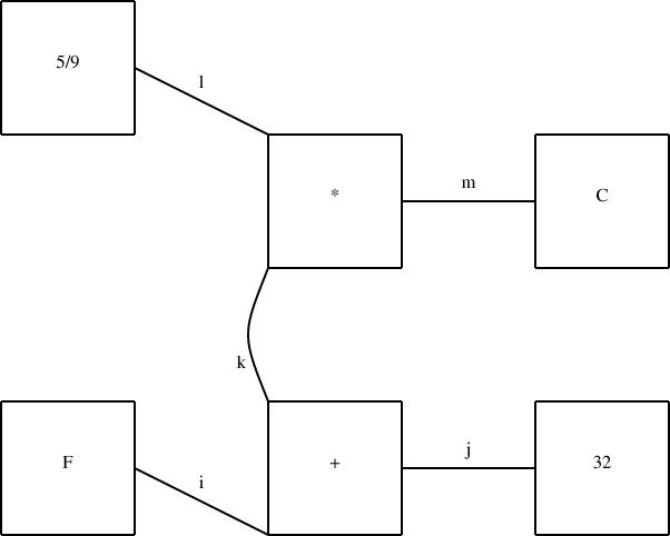
Here was today's surprise. For a long time, my demo diagram has been a rough rendering of one of the figures from Higher-Order Perl:
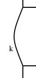
I wanted component k in the middle of the diagram to be a curved line, but since I didn't have curved lines yet, I used two straight lines instead, as shown below:

        define bentline {
          line upper, lower;
          param number depth = 0.2;
          point start, end, center;
          constraints {
            center = upper.end = lower.start;
            start = upper.start;  end = lower.end;
            start.x = end.x = center.x + depth;
            center.y = (start.y + end.y)/2;
          }
        }

        ...

        bentline k;
        label klbl(text="k") = k.upper.center - (0.1, 0);
        ...
        constraints {
          ...
          k.start = plus.sw; k.end = times.nw;
          ...
        }
So I had defined a thing called a bentline, which is a line
with a slight angle in it. Or more precisely, it's two
approximately-vertical lines joined end-to-end. It has three
important reference points: start, which is the top point,
end, the bottom point, which is directly under the top
point), and center, halfway in between, but displaced
rightwards by depth. I now needed to replace this with a curved line. This meant removing all the references to start, end, upper and so forth, since curves don't have any of those things. A significant rewrite, in other words.
But then I had a happy thought. I added the following definition to the file:
        require "curve";
        define bentline_curved extends bentline {
          curve c(N=3);
          constraints {
            c.control[0] = start;
            c.control[1] = center;
            c.control[2] = end;
          }
          draw { c; }
        }
A bentline_curved is now the same as a bentline, but
with an extra curved line, called c, which has three control
points, defined to be identical with start, center,
and end. These three points inherit all the same constraints
as before, and so are constrained in the same way and positioned in
the same way. But instead of drawing the two lines, the
bentline_curved draws only the curve. I then replaced:
bentline k;
with:
bentline_curved k;
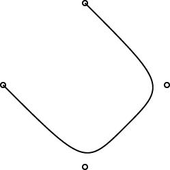
and recompiled the diagram. The result is below:
| | 
|
I didn't foresee this when I designed the linogram language. Sometimes when you try a new kind of program for the first time, you keep getting unpleasant surprises that make you go back and revisit your design, fix problems, try to patch up mismatches, and so forth. The appearance of this sort of pleasant surprise is exactly the opposite sort of situation, and makes me really happy.
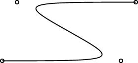
The regular polygons are working pretty well, and the curves are working pretty well. Here are some simple examples:
| 
|
One interesting design problem turned up that I had not foreseen. I had planned for the curve object to be specified by 2 or more control points. (The control points are marked by little circles in the demo pictures above.) The first and last controlpoints would be endpoints, and the curve would start at point 0, then head toward point 1, veer off toward point 2, then veer off toward point 3, etc., until it finally ended at point N. You can see this in the pictures.
This is like the behavior of pic, which has good-looking curves. You don't want to require that the curve pass through all the control points, because that does not give it enough freedom to be curvy. And this behavior is easy to get just by using a degree-N Bézier curve, which was what I planned to do.
However, PostScript surprised me. I had thought that it had degree-N Bézier curves, but it does not. It has only degree-3 ("cubic") Bézier curves. So then I was left with the puzzle of how to use PostScript's Bézier curves to get what I wanted. Or should I just change the definition of curve in linogram to be more like what PostScript wanted? Well, I didn't want to do that, because linogram is supposed to be generic, not a front-end to PostScript. Or, at least, not a front-end only to PostScript.
I did figure out a compromise. The curves generated by the PostScript drawer are made of PostScript's piecewise-cubic curves, but, as you can see from the demo pictures, they still have the behavior I want. The four control points in the small demos above actually turn into two PostScript cubic Bézier curves, with a total of seven control points. If you give linogram the points A, B, C, and D, the PostScript engine draws two cubic Bézier curves, with control points {A, B, B, (B + C)/2} and {(B + C)/2, C, C, D}, respectively. Maybe I'll write a blog article about why I chose to do it this way.
One drawback of this approach is that the curves turn rather sharply near the control points. I may tinker with the formula later to smooth out the curves a bit, but I think for now this part is good enough for beta testing.
        require "polygon";

        polygon t1(N=3), t2(N=3);

        constraints {
          t1.v[0] = (0, 0);
          t1.v[1] = (1, 1);
          t1.v[2] = (2, 3);
          t2.v[i] = t1.v[i-1];
        }
This defines two polygons, t1 and
t2, each with three sides. The three vertices of
t1 are specified explicitly. Triangle
t2 is the same, but with the vertices numbered
differently: t2.v0 =
t1.v2,
t2.v1 =
t1.v0, and
t2.v2 =
t1.v1. Each of the triangles also
has three edges, defined implicitly by the definition in
polygon.lino:
        require "point";
        require "line";

        define polygon {
          param index N;
          point v[N];
          line e[N];
          constraints {
            e[i].start = v[i];
            e[i].end = v[i+1];
          }
        }
All together, there are 38 values here: 2 coordinates for each of
three vertices of each of the two triangles makes 12; 2 coordinates
for each of two endpoints of each of three edges of each of the two
triangles is another 24, and the two N values themselves
makes a total of 12 + 24 + 2 = 38.All of the equations are rather trivial. All the difficulty is in generating the equations in the first place. The program must recognize that the variable i in the polygon definition is a dummy iterator variable, and that it is associatated with the parameter N in the polygon definition. It must propagate the specification of N to the right place, and then iterate the equations appropriately, producing something like:
e0.end = v0+1Then it must fold the constants in the subscripts and apply the appropriate overflow semantics—in this case, 2+1=0.
e1.end = v1+1
e2.end = v2+1
Open figures still don't work properly. I don't think this will take too long to fix.
The code is very messy. For example, all the Type classes are in a file whose name is not Type.pm but Chunk.pm. I plan to have a round of cleanup and consolidation after the 2.0 release, which I hope will be soon.
        define regular_polygon[N] closed {
          param number radius, rotation=0;
          point vertex[N], center;
          line  edge[N];
          constraints {
            vertex[i] = center + radius * cis(rotation + 360*i/N);
            edge[i].start = vertex[i];
            edge[i].end   = vertex[i+1];
          }
        }
The stuff in green is working just right; the stuff in red is not.The following example works just fine:
        number p[3];
        number q[3];
        constraints {
          p[i] = q[i];
          q[i] = i*2;
        }
What's still missing? Well, if you write
        number p[3];
        number q[3];
        constraints {
          p[i] = q[i+1];
        }
This should imply three constraints on elements of p and
q:
p0 = q1
p1 = q2
p2 = q3
The third of these is defective, because there is no q3. If the figure is "closed" (which is the default) the subscripts should wrap around, turning the defective constraint into p2 = q0 instead. If the figure is declared "open", the defective constraint should simply be discarded.
The syntax for parameterized definitions (define regular_polygon[N] { ... }) is still a bit up in the air; I am now leaning toward a syntax that looks more like define regular_polygon { param index N; ... } instead.
The current work on the "arrays" feature is in the CVS repository on the branch arrays; get the version tagged tests-pass to get the most recent working version. Most of the interesting work has been on the files lib/Chunk.pm and lib/Expression.pm.
They include what is probably a better introduction than the one linked above.
        define regular_polygon[N] closed {
          param number radius, rotation=0;
          point vertex[N], center;
          line  edge[N];
          constraints {
            vertex[i] = center + radius * cis(rotation + 360*i/N);
            edge[i].start = vertex[i];
            edge[i].end   = vertex[i+1];
          }
        }
There is a lot of interesting stuff going on here. The [N] in the
define line is a parameter; it means that the definition is
parametrized by N, which can be any non-negative integer. Here
it represents the number of sides in the polygon. So we are defining
a regular polygon with any number of sides. Such a polygon has a
center point and N vertices; also N edges which are
lines.The vertex[i] in the constraints section is a parametrized constraint. It is repeated once for each value of i from 0 up to N-1. cis is a new builtin function: cis(x) simply returns the tuple (cos(x), sin(x)).
The parametrized constraint edge[i].end = vertex[i+1] is particularly interesting. When i = N-1, the subscript in the expression vertex[i+1] is out of range. Parametrized definitions can be either open or closed. For open figures, the out-of-range constraints are just ignored. For closed ones, the subscript is interpreted cyclically, so that the reference to vertex[N] is taken to mean vertex[0] instead. Thus the endpoints of edge[N-1] are vertex[N-1] and vertex[0].
Having made these definitions, we could draw a square and a diamond like this:
        regular_polygon[4]  square(center=(0,0), radius=1),
                           diamond(center=(0,0), radius=1, rotation=45);
A simpler definition defines a spline type:
        define spline[N] open {
          point cp[N];
          draw { &draw_spline; }
        }
The spline has N unconstrained control points; the
draw_spline function is responsible for interpolating the
spline between them.You can follow the progress by watching the CVS repository; see below.
As of 19 August, 2005, version 1.9 is ready. This is feature-complete beta release in anticipation of 2.0. All target features are implemented, including the rudimentary PostScript output generator. There may still be bugs, of course. The 1.90 files in CVS are tagged with tag v1_9; you may also download a .tgz or ZIP archive of the sources.
Output is ugly but functional. Here's an example:
Still to do for 2.0: complete the manual, beta test and fix bugs.
Still to do for the future: see the TODO file. Items marked with * are done; those with o are not done yet.
Sources are available by anonymous CVS at:
cvs -d :pserver:anonymous@plover.com:/data/cvs co linogram
Or you can browse them here:

Return to: Universe of Discourse main page | What's new page | Perl Paraphernalia Higher-Order Perl